A new Demo Mode Course has been created.

Crank Sensor — Tracking down a Misfire

Please note that the Demo Device on the Early Access Version of PicoScope 7 has a problem with its crankshaft waveform. A hall-effect sensor waveform was substituted, but the timing is incorrect. Please use the Stable Version to follow along this discussion.

Introduction

An inductive crankshaft sensor has the advantage that the signal amplitude changes with differing engine speeds. Thus, the relative crank speed could be discerned by variations in the amplitude of the signal. However, that effect is very subtle and not very accurate.

Many newer vehicles now use the more reliable hall sensor which produces a constant amplitude digital signal, usually 5 V. This means that new techniques are required to examine relative engine speed.

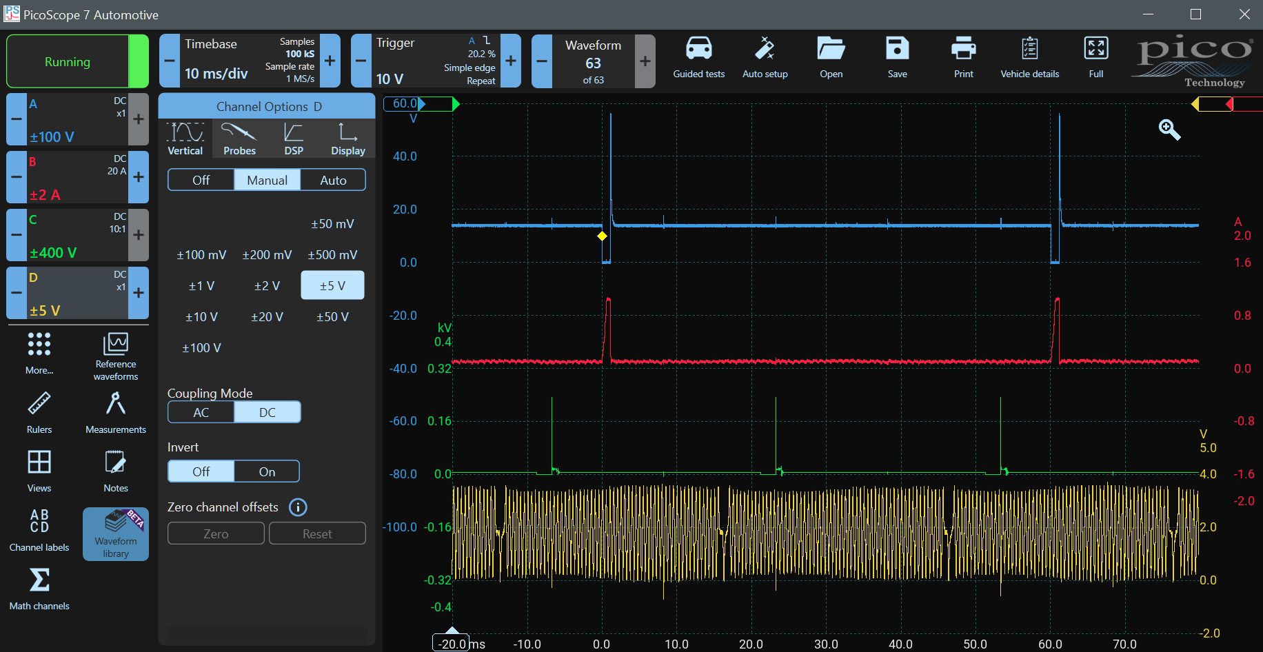
Enable Channel D to see the crankshaft sensor output.

Configuring Channel D

Click on the Channel D Control and set it up as follows:

• Vertical Tab
  • Select ±5V
  • Coupling DC
  • Invert Off
• Probes Tab
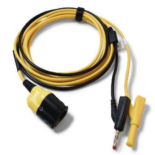
  • Select X1 ( Test Lead)
• DSP Tab
  • Low-Pass Filter Off
  • Resolution-Enhance 12 bits
• Display Tab
  • Scale x0.5
  • Offset -80%

Notice that we have set the crank sensor voltage to ±5V to maximise its resolution and used scaling to reduce its size on the display. If you zoom in, you will have the maximum resolution available to reveal fine signal detail.

DSP Filtering

Many automotive signals have high-frequency noise superimposed on them because of interference from adjacent wiring, and automotive signal wires are rarely shielded. High-frequency noise can distort and mask signals, but you can use filtering to reduce that noise. Notice that the crank signal has low-going spikes that coincide with ignition ionisation spikes. Whilst these are inconsequential here, we will filter them out using a Low Pass DSP Filter as an exercise.

Click on the Channel D control and select DSP. DSP means digital signal processing. PicoScope uses DSP to filter waveforms and to enhance resolution. Set the Low Pass Filter to 100 kHz and make it active. You will see very little change to the signal because 100 kHz is higher than the frequency components in the waveform.

Gradually reduce the frequency using the left - control until you start to see the amplitude of the wave start to reduce. By the time you get to 10 kHz, the ignition spikes will have almost disappeared, but the amplitude of the signal will not have changed. When you get to about 8 kHz, the signal will start getting smaller. This means that you have gone too far, and you are changing the signal you are trying to measure. Set the filter back to 12 kHz. The spikes induced by the ignition have almost disappeared.

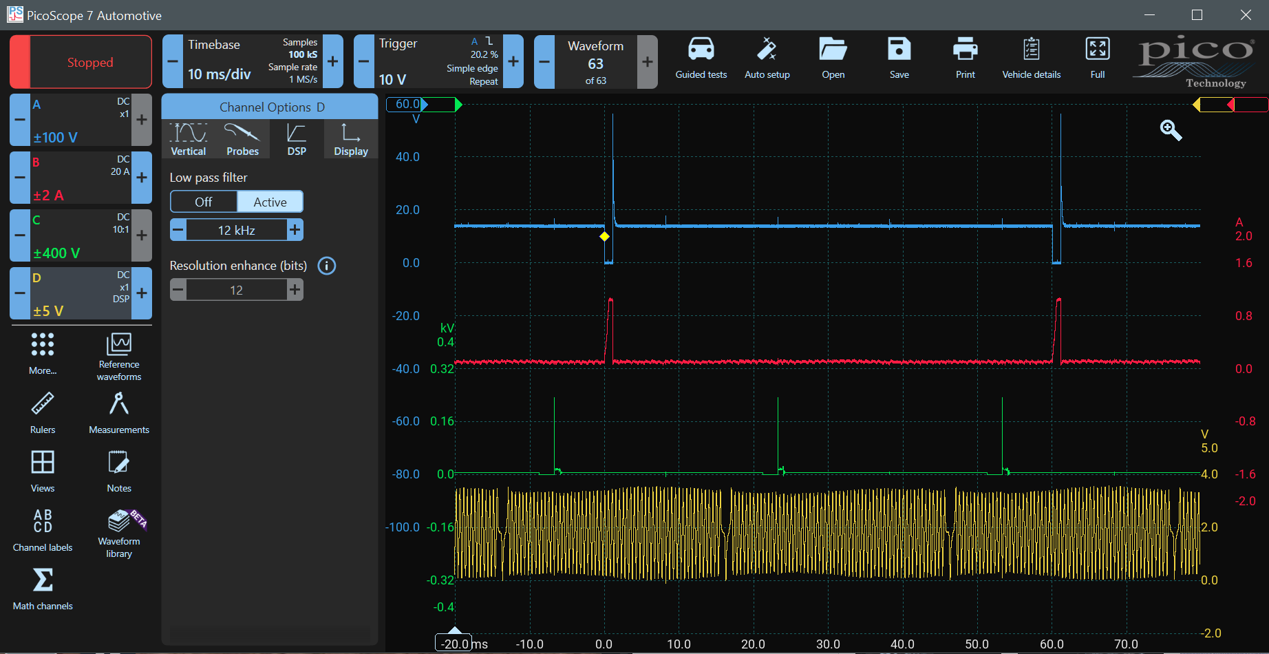
Now stop the scope and set the filter to off. Notice that the signal was captured and stored without filtering, and the DSP filter only affected the display. All the signal information remains intact.

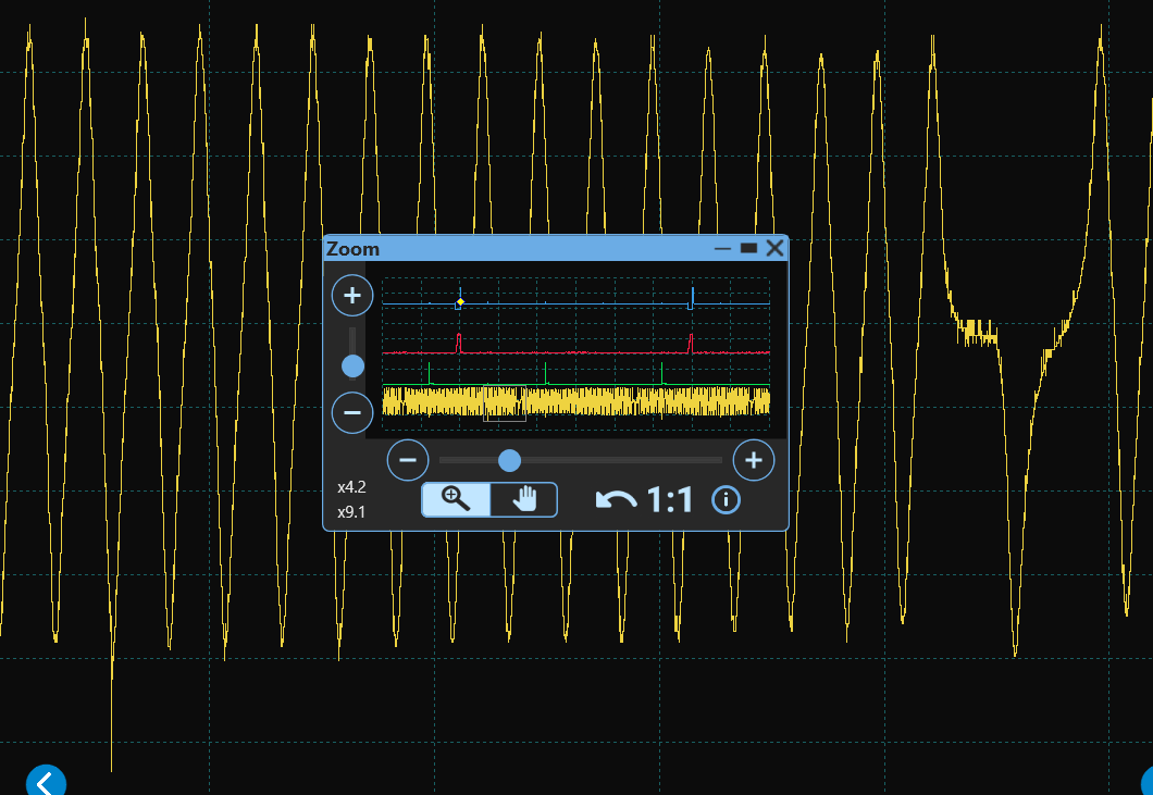
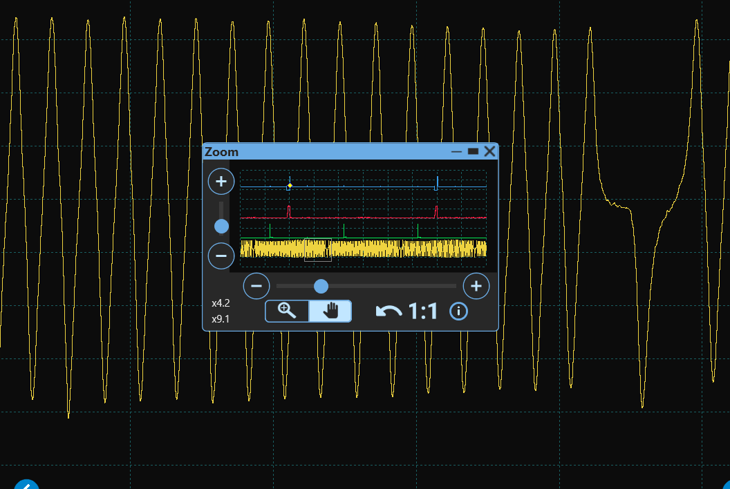
Zoom into the waveform including one of the ignition disturbances and a missing tooth (see the images below). Examine the waveform with the filter off and note the resolution or detail that is available. Make the filter active and notice how the noise and ignition spikes are reduced.

Crank Sensor

The crank sensor is a definitive source of information about the absolute rotational position of the engine. Its timing is unaffected by factors such as VVT or ignition advance. The missing tooth (or teeth) is used as an index.

PicoScope Waveform Library

Remember that the position of the missing tooth does not necessarily line up with a particular engine state (such as TDC) - it is somewhat random from engine to engine. Therefore, the PicoScope waveform library is a valuable resource. Once you have a PicoScope, you can download known good waveforms and compare them with the engine you are working on.

Using rulers

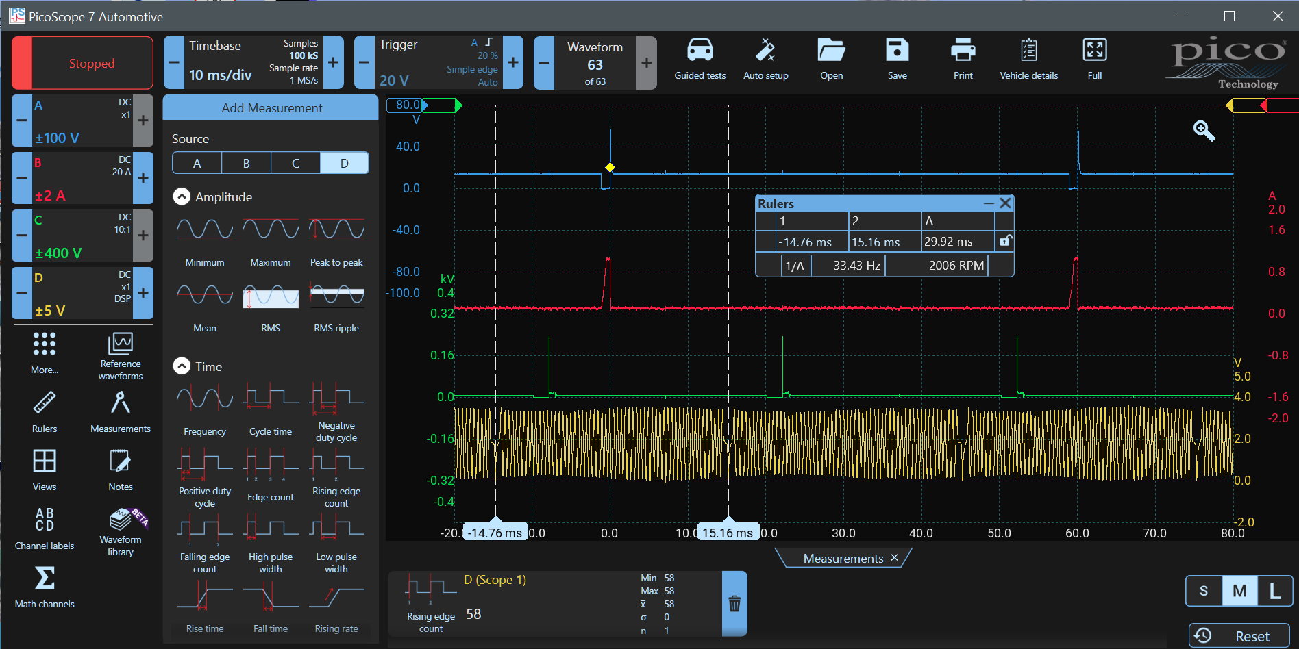
Earlier, we measured the interval between injector pulses to determine RPM. That is not the most accurate procedure because the ECU can vary the position of the injection events. Using ignition also provides a good approximation, but ignition events are also not fixed. Drag in two rulers from the left and use Zoom to align them accurately with the negative peaks on two missing teeth intervals. The engine Speed in RPM will be displayed — 2006 RPM.

Using Measurements to Count

You can physically count the teeth on the crank reluctor, but it is easier to get PicoScope to do that for you. Click on the 'Measurements' Icon (click More if it isn't displayed). Choose Channel D and rising (or falling) Edge Count (not Edge Count as it will double your result as it counts both edges). Click on the Edge Control that appears at the bottom of the screen and change the Section to 'between rulers' and select Automatic. You will see that 58 edges are counted. There are two missing teeth, so the crank sensor has 60 tooth positions (including the missing teeth).

Finding a Misfire

When each engine cylinder compresses the air-fuel mixture prior to ignition, a load is exerted that slows the engine slightly. When ignition takes place (just before TDC), the engine speeds up during the power stroke. This effect can be seen by the subtle changes in amplitude of the inductive crank sensor. However, bear in mind that this isn't very reliable because the distance between the sensor and teeth can alter the amplitude significantly. If a hall-effect sensor is used, there is no change in amplitude because the signal is digital (usually a square wave between 5 V and 0 V).

The engine should accelerate and decelerate at regular intervals at each power stroke. A four-cylinder 4-stroke engine has two power strokes per revolution and thus has two accelerations and decelerations. As an aside, when you use PicoScope for NVH testing, an E2 (two disturbances per engine revolution) vibration is detected when accelerating in a 4-cylinder vehicle, an E3 vibration in a six-cylinder engine, and so on.

When a misfire occurs, the engine fails to accelerate during one or more power strokes. The PicoScope can detect and display the misfire reliably.

Click on the Math Channels icon (click More if it is not displayed). Click the + Add Icon and type the formula in the text box at the top Crank(D, 60). This means the Crank Signal is on Channel D and there are 60 tooth positions around the crank reluctor (flywheel). Click Next

Change the colour to something distinct — I used mauve. We know that the engine speed is 2006RPM (we measured it above), so set the display range just above and below that value. I used 2250 RPM Max and 1750RPM Min. Note that the entry box may insist on krpm so enter 2250 as 2.250krpm. Click Finish and the engine speed will be displayed. You might want to rearrange your waveforms.

Cleaning up the RPM Waveform

You can clearly see the trends — the engine speeds up after ignition and slows just before it. However, the Crank Speed Waveform isn't very smooth and the engine is unlikely to change speed at the rate of the high-frequency noise on the signal. The Inductive Crank signal is analogue, and the thresholds aren't very accurate — the amplitude of the waveform is variable. Hall effect sensors tend to be more accurate.

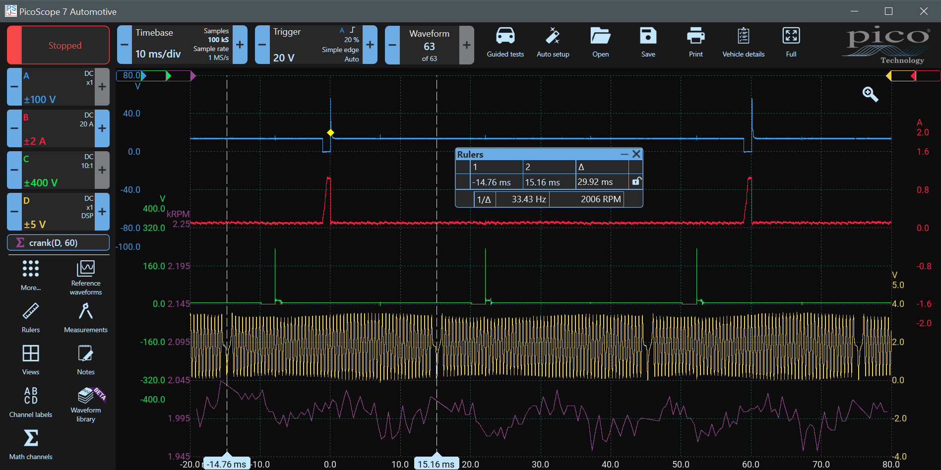
We can filter out a lot of the noise by modifying our math channel formula and adding a filter. To show the improvement, we will add another filtered math channel.

Click the Math Channels Icon and click + Add. Type the formula LowPass(crank(D, 60), 130). This means 'take the Crank Signal on Channel D which has 60 tooth positions and apply a low-pass filter which removes frequencies above 130 Hz'.

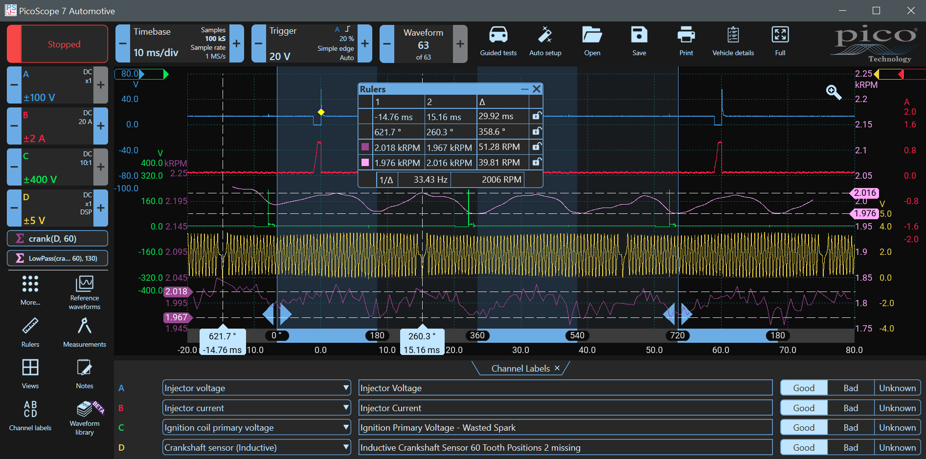
Why 130 Hz? If you look at the rulers-box, you will see that 2006 RPM translates to 33.43 Hz. There are two combustion events per revolution, so the frequency of combustion events is 66.86 Hz. We chose a cutoff frequency that is about twice the frequency of interest. Click Next.

Choose another distinct colour, I chose pink and specify the same range as above - 2250 to 1750 RPM.

Now the acceleration and deceleration are obvious and occur after each ignition event. No misfires have been detected.

Visualising the 4-stroke Cycle

Click the Rulers-Icon and turn the Phase Rulers on. The Preset Boundaries should be 720 degrees (two revolutions), and partitions should be 4. Use Zoom to position the left phase ruler one crank peak (about 6 degrees) after the end of the first ignition waveform on Channel C.

Skip the next ignition event and use Zoom to position the right phase ruler one crank peak (about 6 degrees) after the end of the third ignition waveform on Channel C. That is approximately TDC for that cylinder. The ruler shading delineates the four phases of the four-stroke cycle.

The injection event in the first phase - inlet (0° to 180°) - is followed by a compression phase (180° to 360°) with an ignition event just before TDC. This is followed by a power stroke (360° to 540°) — note the acceleration after the ignition event. The exhaust phase follows at 540° to 720°, and the cycle begins again with an inlet phase.

In the above image, the sample count is only 100 kS. If you increase the sample rate, the filtered waveform will change and more high-frequency components will appear. Remember that Sample Rate can affect filtering. You may need to adjust your filter frequency to compensate.

Remember to provide Channel Labels Click Channel Labels to open them so that you can understand what you have measured if you need to return to the waveform after saving it. Save your waveforms.

We hope you have enjoyed the Demo Mode Course. There is much more to be learned in our Top-10 Tests Presentation. You can use PicoScope 7 Software (a PicoScope isn't required) to try many of the tests yourself.